Adjacency Array

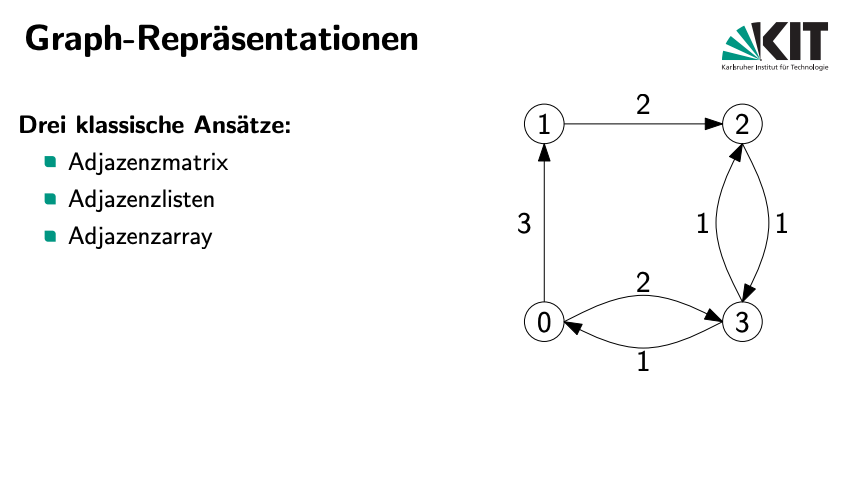
While reviewing the slides from a KIT lecture titled “Algorithms for Route Planning,” I came across a graph representation that I hadn’t encountered before: the adjacency array. The lecture showed the adjacency array side by side with the adjacency list, so it was clear that they were two different ways to represent a graph.

Like most people, I turned to Google and searched for “adjacency array.” However, there weren’t many resources available in English, except for one PDF from MPI (Max Planck Institute): source link. The description and example there were initially unclear to me. But after some help from ChatGPT, I was able to grasp the concept.

What Is an Adjacency Array?

Before diving into adjacency arrays, let’s briefly review two common graph representations:

• Adjacency Matrix: This matrix uses the combination of row $r$ and column $c$ to represent whether there’s an edge from node $r$ to node $c$.
• Adjacency List: This list uses the index $i$ to represent a start node and links to a list of nodes that it connects to.

Now, an adjacency array is a more space-efficient way to represent a graph, using two arrays. Let’s break it down.

1. The Edge Array (E): This array stores the destination nodes (to-nodes) and is ordered by the source node (from-node). For example, if we have the graph below, the edge array E might look like this:

   \[E = [2, 4, 3, 1, 2, 0]\]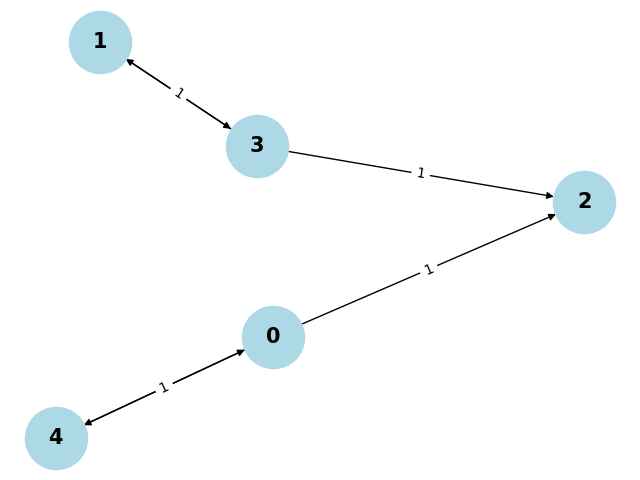

   

   This means:

   • Node 0 connects to Node 2 and Node 4
   • Node 1 connects to Node 3
   • Node 3 connects to Node 1 and Node 2
   • Node 4 connects to Node 0

2. The Vertex Array (V): The second array, $V$, uses the index to represent the source node $i$. The value at $V[i]$ indicates the index of the first connection for node $i$ in the edge array $E$. So for our example, the vertex array $V$ would be:

   \[V = [0, 2, 3, 3, 5]\]

How to Use the Arrays

To find the edges from node 0, for instance, you look at the elements in $E$ between $V[0]$ and $V[1] - 1$. So, for node 0, the connections are found between $E[0]$ and $E[1]$, which gives us Nodes 2 and 4.

• Node 2 has no outgoing edges (out-degree is 0), and since $V[2]$ and $V[3] - 1$ don’t form a valid range, we know Node 2 doesn’t connect to any other node.

• Node 4 is the last node in the vertex array $V$. To handle this case, a dummy element is often added to the end of $V$. This extra element ensures we can handle the last node in a consistent way. For this graph, $V$ would become:

  \[V = [0, 2, 3, 3, 5, 6]\]

This dummy element helps define the range of connections for the last node in the graph.

Complexity and Storage

For a directed graph with $n$ nodes and $m$ edges, where the edges are represented as a sequence, constructing an adjacency array requires sorting the source nodes, which has a time complexity of $O(m\log{}m)$.

In terms of storage, the adjacency array uses $O(n+m)$ space, making it more efficient than some other representations, particularly for sparse graphs.

However, since this data structure relies on two arrays, adding or removing an edge is not efficient—it requires $O(n)$ time complexity because inserting or deleting elements in arrays involves shifting data. As a result, adjacency arrays are best suited for static graph representations, where the structure of the graph remains unchanged after it is created.