This post is related with the seminar Mathematics of machine learning that I am taking this winter semester. In the seminar of this semester, the main topics is about sampling techniques. I am interested in this area. And since I am about to graduate and have plenty of free time. I decided to write some posts and also do some programming about what I learned in the seminar.

Problem scenario

Let’s go back to the topic rejection sampling. It is a technique to generate observations from a distribution. We assume that there is a probability distribution $p(z)$. We want to sample from it.

Here is the description of $p(z)$ in [1], we are easily able to evaluate $p(z)$ for any given value of z, up to some normalizing constant Z, so that

\[p(z) = \frac{1}{Z_p}\tilde{p}(z)\]

The interesting question is when we are in this situation. A known $\tilde{p}(z)$ is equal to some certain constant $Z_p$ times $p(z)$.

Actually Bayes' theorem gives us one example. The evidence $p(x)$ is a constant. The posterior $p(\theta | x)$ is proportional to the prior $p(\theta)$ times likelihood $p(x | \theta)$ [2].

\[p(\theta | x) = \frac{p(x | \theta)p(\theta)}{p(x)}\]

Definitions and assumptions

Assuming that we can only sample from some standard distributions $q(x)$, for example Gaussian distribution and uniform distribution. We call it proposal distribution.

We define that the probability distribution that we want to take samples from is $p(z)$, which is a complicated distribution. We have $\tilde{p}(x) = Z_p* p(z)$.

Then we introduce a constant $k$ that for all $z$, $kq(z) \geq \tilde{p}(z)$. $kq(z)$ is called envelope function or comparision function.

Algorithm details

The rejection sampling algorithm is:

1. Take a sample $z_0$ from distribution $q(z)$.

2. Calculate the value $kq(z_0)$ and $\tilde{p}(z_0)$

3. Take a sample $u_0$ from uniform distribution $U[0, kq(z_0)]$.

4. If $u_0 > \tilde{p}(z_0)$:

       Reject and back to step 1

       else:

            $u_0$ is a sample from $p(z)$

Proof

Based on the previous algorithm detail section and law of total probability, we know that the probability of accept (abbreviated as $A$ in the following equations) is

\[p(A) = \int p(A | z) q(z) dz = \int \frac{\tilde{p}(z)}{kq(z)}q(z) dz = \frac{Z}{k}\]

Using Bayes’ theorem, we have

\[p(z | A) = \frac{p(A | z) q(z)}{p(A)} = p(z)\]

So the probability density or probability mass of accepted sample $z$ equal to the sample from desired probability distribution $p(z)$.

Experiments of implementation

The figure shown below is the overview of rejection sampling scenario.

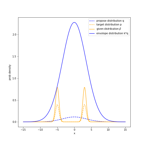
The orange dashed line is the probability distribution $p(x)$ that we want to sample from, which is a mixture of Gaussian. \(p(x) = \theta_1 N(\mu_1, \sigma_1^2) + \theta_2 N(\mu_2, \sigma_2^2)\) where $\theta_1 = 0.5, \mu_1 = -5, \sigma_1 = 0.5$ and $\theta_2 = 0.5, \mu_2 = -5, \sigma_2 = 0.5$.

I chose small s.t.d for the target distribution so that most of the samples from this distribution will be clustered at the two means $\mu_1$ and $\mu_2$.

The given distribution $\tilde{p}(x) = 2 * p(x)$. So the propose distribution $q(x)$ is a Gaussian distribution with $\mu = 0$ and $\sigma = 3.5$. Since the $Z = 2$, to make the envolope function covers the given distribution, $k = 20$.

From the figure above, we see that the blue curve representing envolope distribution $k * q(x)$ does cover the given distribution.

The figure below is 300 samples from $p(x)$. Clearly, most samples are centered at the $x=-5$ and $x=3$. To make sure that the implementation is correct, we fit a mixture of Gaussian model from sklearn to these points. The result of fitting shows that the sampled mean is $-4.998$ and $2.999$. The sampled variance is $0.2525$ and $0.2434$.

More detailed code is here.

References

[1] Bishop, Christopher M. Pattern recognition and machine learning, 2006.

[2] Lee, Peter M. Bayesian statistics. Arnold Publication, 1997.